fd471ced3e24422db5442242d8dc4ce6

Tutorial: basics of FARGOpy

[ ]:

try:
    from google.colab import drive
    %pip install -Uq git+https://github.com/seap-udea/fargopy
except ImportError:
    print("Not running in Colab, skipping installation")
    %load_ext autoreload
    %autoreload 2
!mkdir -p ./gallery/

Not running in Colab, skipping installation

If you are in Google Colab, install the latest version of the package:

For this tutorial you will need the following external modules and tools:

[ ]:

import fargopy as fp
import numpy as np
import matplotlib.pyplot as plt
from celluloid import Camera
from IPython.display import HTML
from tqdm import tqdm

Running FARGOpy version 1.1.0. A major refactor has been done in versions 1.1.X. Please check the documentation for more information.

Let’s `FARGOpy`

First we need the data. Let’s download a precomputed simulation. Check the list:

[ ]:

fp.Simulation.list_precomputed()

fargo:
        Description: Protoplanetary disk with a Jovian planet [2D]
        Size: 55 MB
p3diso:
        Description: Protoplanetary disk with a Super earth planet [3D]
        Size: 220 MB
p3disoj:
        Description: Protoplanetary disk with a Jovian planet [3D]
        Size: 84 MB
fargo_multifluid:
        Description: Protoplanetary disk with several fluids (dust) and a Jovian planet in 2D
        Size: 100 MB
binary:
        Description: Disk around a binary with the properties of Kepler-38 in 2D
        Size: 140 MB
pds70iso:
        Description: PDS-70c - isothermal protoplanetary disk and circumplanetary disk in [3D]
        Size: 2940 MB

Download, for instance, the 2D simulation of a disk with a Jovian planet:

[ ]:

simpath = fp.Simulation.download_precomputed('p3disoj')

Precomputed output directory '/tmp/p3disoj' already exist

Once download it, we need to connect a Simulation with the directory with the simulation results:

[ ]:

sim = fp.Simulation(output_dir=simpath)

Your simulation is now connected with '/Users/jzuluaga/fargo3d/'
Now you are connected with output directory '/tmp/p3disoj'
Found a variables.par file in '/tmp/p3disoj', loading properties
Loading variables
85 variables loaded
Simulation in 3 dimensions
Loading domain in spherical coordinates:
        Variable phi: 128 [[0, np.float64(-3.117048960983623)], [-1, np.float64(3.117048960983623)]]
        Variable r: 64 [[0, np.float64(0.5078125)], [-1, np.float64(1.4921875)]]
        Variable theta: 32 [[0, np.float64(1.4231400767948967)], [-1, np.float64(1.5684525767948965)]]
Number of snapshots in output directory: 11
Planets found in summary.dat:
  Name: Jupiter, Initial pos: [1.0, 0.001, 0.0], Mass: 0.001

Let’s read the field we want to animate, eg. the gas density. It is important to notice that we will animate the field in a slice corresponding to \(z=0\):

[ ]:

fields_spherical = sim.load_field(
    fields='gasdens',
    snapshot=[1, sim.nsnaps-1],
    coords='spherical',
    slice='theta=1.56'
)

fields_cartesian = sim.load_field(
    fields='gasdens',
    snapshot=[1, sim.nsnaps-1],
    coords='cartesian',
    slice='theta=1.56'
)

And the plot can be done using:

[ ]:

snapshot = 5

phi = fields_spherical.var1_mesh[snapshot]
r = fields_spherical.var2_mesh[snapshot]

x = fields_cartesian.var1_mesh[snapshot]
y = fields_cartesian.var2_mesh[snapshot]

gasdens_plane = fields_cartesian.gasdens_mesh[snapshot]

x.shape, y.shape, gasdens_plane.shape, r.shape, phi.shape

((64, 128), (64, 128), (64, 128), (64, 128), (64, 128))

[ ]:

plt.close('all')
fig,axs = plt.subplots(1,2,figsize=(12,6))
cmap = 'turbo'

ax = axs[0]
ax.pcolormesh(phi*fp.RAD,r*sim.UL/fp.AU,gasdens_plane*sim.USIGMA,cmap=cmap)
ax.set_xlabel('$\phi$ [deg]')
ax.set_ylabel('$r$ [au]')

ax = axs[1]
c = ax.pcolormesh(x*sim.UL/fp.AU,y*sim.UL/fp.AU,gasdens_plane*sim.USIGMA,cmap=cmap)
ax.set_xlabel('$x$ [au]')
ax.set_ylabel('$y$ [au]')
ax.axis('equal')
fp.Plot.fargopy_mark(ax, frac=1/4)

axc = fig.colorbar(c)
axc.set_label("$\Sigma$ [g/cm$^2$]")
plt.savefig('gallery/fargopy-tutorial-animations_0.png') # Save figure

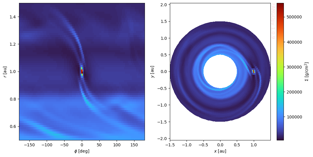
../_images/examples_fargopy-tutorial-basics_17_0.png

Notice that we have used the units of the simulation to convert all quantities from simulation units to physical units.

Now, to create the animation we repeat the previous procedure at each snapshot:

[ ]:

plt.ioff()
fig,axs = plt.subplots(1,2,figsize=(12,6))
cmap = 'turbo'

# Create a Celluloid camera
camera = Camera(fig)

for snapshot in tqdm(range(sim.nsnaps-1)):
    # For each snapshot get the desnity and meshslice it
    phi = fields_spherical.var1_mesh[snapshot]
    r = fields_spherical.var2_mesh[snapshot]
    x = fields_cartesian.var1_mesh[snapshot]
    y = fields_cartesian.var2_mesh[snapshot]
    gasdens_plane = fields_cartesian.gasdens_mesh[snapshot]

    ax = axs[0]
    ax.pcolormesh(phi*fp.RAD,r*sim.UL/fp.AU,gasdens_plane*sim.USIGMA,cmap=cmap)
    ax.set_xlabel('$\phi$ [deg]')
    ax.set_ylabel('$r$ [au]')

    ax = axs[1]
    c = ax.pcolormesh(x*sim.UL/fp.AU,y*sim.UL/fp.AU,gasdens_plane*sim.USIGMA,cmap=cmap)
    ax.set_xlabel('$x$ [au]')
    ax.set_ylabel('$y$ [au]')
    ax.axis('equal')
    fp.Plot.fargopy_mark(ax)

    # Take a snapshot of the figure
    camera.snap()

# Create the animation object
animation = camera.animate()
plt.ion()
plt.savefig('gallery/fargopy-tutorial-animations_1.png') # Save figure
animation.save('gallery/fargopy-tutorial-animations_2.gif', writer='pillow') # Save animation

100%|██████████| 10/10 [00:00<00:00, 288.47it/s]

Once you have snapped all the frames we can create the animation, save it and/or visualize it:

[ ]:

HTML(animation.to_html5_video())

Save it into a gif:

[ ]:

animation.save('gallery/fargo.gif', fps=5)

And that’s it!

Animations preview

Since the animations in this notebook will not be displayed on the web we include here the animation figures which are available in the GitHub repository:

Powered by fargopy. For more examples see fargopy GitHub repo.

Tutorial: basics of FARGOpy

Let’s FARGOpy

Animations preview

Let’s `FARGOpy`